
By: Kristoffer Hultgren
Karlstad University
Faculty of Technology and Science
Department of Physics
Course: Analytical Mechanics (FYSCD2)
Examiner: Prof. Jürgen Fuchs
January 5, 2007
Pulsars are rapidly rotating highly magnetized neutron stars and are formed by
a Type II supernova explosion. A Type II supernova is characterized by having
a spectrum with prominent hydrogen lines and is produced by a core collapse in
a massive star whose outer layers were largely intact. A small, compact star
may be left. Its gravity is then so strong that the electrons have been forced
into the protons in the atomic nuclei and formed neutrons. The star has an
enormous density but though only about 20 km in diameter, yet it weighs at
least as much as our Sun. When charged particles are accelerated near a
magnetized neutron star's magnetic poles, two oppositely directed beams of
radiation are created (as shown in figure 1). The
fastest pulsars spin several hundreds of revolutions per second and if the
star's magnetic axis is tilted at an angle from the axis of rotation, the beam
sweeps around the sky as the star rotates. If the Earth lies in the path of
one of these beams, we detect radiation that appears to pulse on and off. The
period of the pulses is therefore simply the rotation period of the neutron
star.
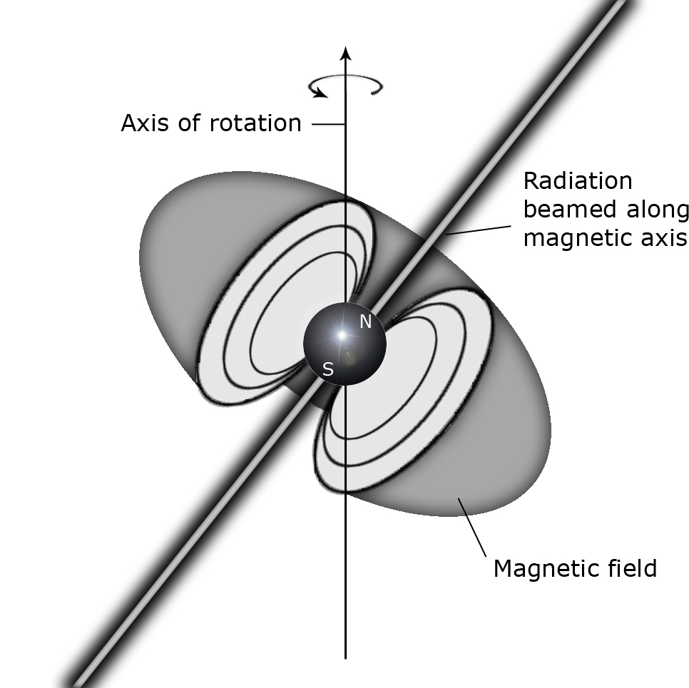
Figure 1: A rotating, magnetized neutron star.
About half of the visible stars in the night sky are not isolated individuals. Instead they are multiple-star systems, in which two or more stars orbit each other, called binary systems. These stars orbit each other because of the mutual gravitational attraction and, in the Newtonian thinking, their orbital motions obey Kepler's third law. If the orbit that one star appears to describe around the other is considered, Kepler's third law for binary star systems can be written as
![]() (1.1)
(1.1)
where ![]() and
and ![]() are the masses of the stars,
are the masses of the stars, ![]() is the semi-major axis of one star's orbit around the other and
is the semi-major axis of one star's orbit around the other and ![]() is the orbital period.
is the orbital period.
About 4% of all known pulsars in the galactic disc are members of binary systems. Their orbiting companions are either white dwarfs, main sequence stars or other neutron stars. If two pulsars are massive and move around each other in tight orbits, they lose energy through a process called gravitational radiation. This is a prediction of Einstein's general theory of relativity and will briefly be discussed in section 4. As a result the two pulsars spiral toward each other and eventually collide, a process that may play an important role in seeding the interstellar medium with the building blocks of planets.
Soon after their discovery it became clear that pulsars are excellent
celestial clocks. The period can be measured to one part in
![]() over a few months leading to a source for applications used as time keepers
and probes of relativistic gravity, like Gravity Probe
B Note_1 .
over a few months leading to a source for applications used as time keepers
and probes of relativistic gravity, like Gravity Probe
B Note_1 .
In order to model the rotational motion of the neutron star, we need to
measure the time of arrival in an inertial frame. An observatory on Earth
experiences accelerations with respect to the neutron star due to the Earth's
rotation and orbital motion around the Sun and is therefore not an inertial
frame. The barycenter (center of gravity) of the solar system can, to a very
good approximation, be regarded as an inertial frame. The transformation is
summarized as the difference between the barycentric time of arrival
![]() and the observed time of arrival
and the observed time of arrival
![]() and can be written
as
and can be written
as
![]() (1.2)
(1.2)
where
![]() is the position of the observatory with respect to the barycenter,
is the position of the observatory with respect to the barycenter,
![]() is a unit vector in the direction of the pulsar at a distance
is a unit vector in the direction of the pulsar at a distance
![]() and
and
![]() is the speed of light. The terms
is the speed of light. The terms
![]() and
and
![]() represents
the Einstein and Shapiro corrections due to general relativistic time delays
in the solar system and will be discussed further in section 3.1. Measurements
can be carried out at different observing frequencies with different
dispersive delays (different frequencies propagate at different group
velocities) so the times of arrival are generally referred to the equivalent
time that would be observed at infinite frequency. This transformation is the
term
represents
the Einstein and Shapiro corrections due to general relativistic time delays
in the solar system and will be discussed further in section 3.1. Measurements
can be carried out at different observing frequencies with different
dispersive delays (different frequencies propagate at different group
velocities) so the times of arrival are generally referred to the equivalent
time that would be observed at infinite frequency. This transformation is the
term
![]() .
.
The ordinary non-relativistic two-body problem can be divided in two sub-problems. The first being the derivation of the orbital equations of motion for two gravitationally interacting bodies, and the second being the solution of these equations of motion. The first sub-problem can be simplified by approximating the orbital equations of motion of the bodies by the equations of motion of two point masses. By doing this, the second sub-problem can be exactly solved.
The two-body problem in General Relativity is not at all well posed and since
the equations of motion are contained in the gravitational field equations it
is not a simple thing to separate the problem in two sub-problems as in the
non-relativistic case. Even if one could achieve such a separation and derive
some equations of orbital motion for the two bodies, these equations would not
be ordinary differential equations but some kind of
retarded-integro-differential
system Note_2 . This
system can however be transformed into ordinary differential equations and,
for widely separated, slowly moving, strongly self-gravitating bodies,
expanded in power series of
![]() .
For the first post-Newtonian approximation, i.e. the first relativistic
corrections to Newtons first law, the orbital equations of motion for these
bodies depend only on two parameters having the dimensions of mass and are
identical to the equations of motion for weakly self-gravitating bodies. At
this point, the first sub-problem is managed and the second sub-problem is
solved at the first post-Newtonian level.
.
For the first post-Newtonian approximation, i.e. the first relativistic
corrections to Newtons first law, the orbital equations of motion for these
bodies depend only on two parameters having the dimensions of mass and are
identical to the equations of motion for weakly self-gravitating bodies. At
this point, the first sub-problem is managed and the second sub-problem is
solved at the first post-Newtonian level.
The extremely precise tracking of the orbital motion of the Hulse-Talyor pulsar PSR1913+16 made it necessary to work out explicitly all the post-Newtonian effects in the motion. This section reviews the main parts of the method for solving this motion presented by Damour and Deruelle in [4].
The (first) post-Newtonian orbital equations of motion of a binary system can
be derived from a Lagrangian with positions of the centers of mass
![]() and
and
![]() of the two bodies:
of the two bodies:
with
and

where
![]() and
and
![]() are the mass parameters of the bodies,
are the mass parameters of the bodies,
![]() ,
,
![]() ,
,
![]() ,
,
![]() is the velocity of light and
is the velocity of light and
![]() is Newton's constant. The notations
is Newton's constant. The notations
![]() and
and
![]() have been used. The total linear momentum of the system can be shown to be
constant and is given
by
have been used. The total linear momentum of the system can be shown to be
constant and is given
by
![]()
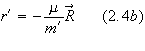
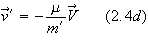
In a post-Newtonian center of mass frame where
![]() the center of mass expressions are given by
the center of mass expressions are given by
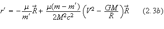
It
can even be shown to be sufficient to use the non-relativistic center of mass
expressions given by
![]()
![]()
where
![]() ,
,
![]() and
and
![]() .
The problem has now reduced to the much more simpler problem of solving the
relative motion in the post-Newtonian center of mass frame. The resulting
relative Lagrangian can then
.
The problem has now reduced to the much more simpler problem of solving the
relative motion in the post-Newtonian center of mass frame. The resulting
relative Lagrangian can then
be shown
to be given by
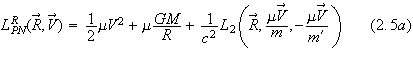
with
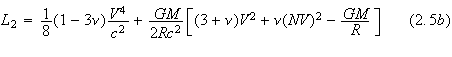
where
we have introduced
![]() .
The Lagrangian in equation (2.5) was obtained by Infeld and Plebanski in [3].
.
The Lagrangian in equation (2.5) was obtained by Infeld and Plebanski in [3].
By using an approach closely following the standard methods for solving a
non-relativistic two-body problem and by using polar coordinates,
![]() and
and
![]() ,
in the plane in which the motion takes place one can finally find the
post-Newtonian equation of radial motion
,
in the plane in which the motion takes place one can finally find the
post-Newtonian equation of radial motion
and
the post-Newtonian equation of angular motion
where
the coefficients
![]() ,
,
![]() ,
,
![]() ,
,
![]() ,
,
![]() and
and
![]() are the following polynomials:
are the following polynomials:
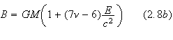
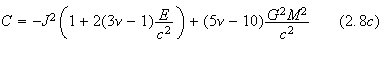
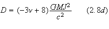
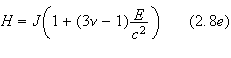
Here,
the center of mass energy
![]() and angular momentum
and angular momentum
![]() is given by
is given by
![]()
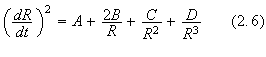
To solve the equation of radial motion we will now reduce the problem to the
integration of an auxiliary, i.e. a "helping", non-relativistic radial motion.
Using the change of variable
where
![]() .
Using the fact that
.
Using the fact that
![]() is of order
is of order
![]() and that we can neglect terms of order
and that we can neglect terms of order
![]() ,
replacing (2.11) in (2.6) gives us
,
replacing (2.11) in (2.6) gives us
where
![]() .
.
The
solution of (2.12) is retrieved by introducing a parametrization by means of
the eccentric anomaly
![]() .
The eccentric anomaly is the angle between the direction of periapsis and the
current position of an object on its orbit, projected onto the ellipse's
circumscribing circle perpendicularly to the major axis, measured at the
centre of the ellipse (figure
2).
.
The eccentric anomaly is the angle between the direction of periapsis and the
current position of an object on its orbit, projected onto the ellipse's
circumscribing circle perpendicularly to the major axis, measured at the
centre of the ellipse (figure
2).
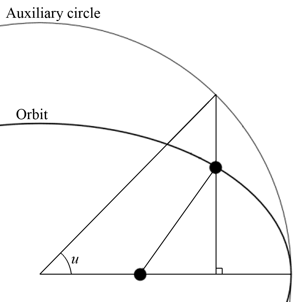
Figure 2: Eccentric anomaly.
The solution is given
by
![]()
![]()
where
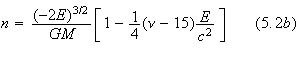
In
these formulas,
![]() represents the mean motion and
represents the mean motion and
![]() is the relative semi-major axis of the orbit. Furthermore,
is the relative semi-major axis of the orbit. Furthermore,
![]() represents the time eccentricity and
represents the time eccentricity and
![]() represents the relative radial eccentricity. The
eccentricity may be interpreted as a measure of how much this shape deviates
from a circle and the appearance of two different eccentricities is the main
difference between the relativistic radial motion and the non-relativistic
one. The relationship between these two is given by
represents the relative radial eccentricity. The
eccentricity may be interpreted as a measure of how much this shape deviates
from a circle and the appearance of two different eccentricities is the main
difference between the relativistic radial motion and the non-relativistic
one. The relationship between these two is given by
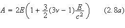
By
using (2.8),
![]() ,
,
![]() ,
,
![]() and
and
![]() can be written in terms of
can be written in terms of
![]() and
and
![]() :
:
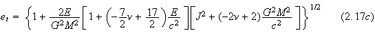
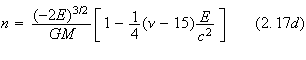
Here
one sees that both the semi major axis and the mean motion depend only on the
center of mass energy. This means that the well-known result of the Newtonian
elliptic motion is still valid at the post-Newtonian level. In fact, the same
is also true for the period of the orbit,
![]() .
.
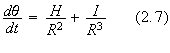
The problem of solving the equation of angular motion can, just as before, be
reduced to the integration of an auxiliary non-relativistic angular motion.
Let us make the following change of variable:
Replacing
(2.18) in (2.7) gives us then
where
we can use
![]() as
as
![]()
with
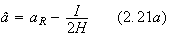
Using
(2.13) we see that
![]()
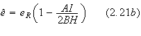
and
hence
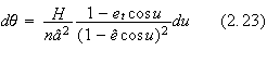
Comparing
(2.16) and (2.21b) we see that
![]() and
and
![]() differ only by a small term of order
differ only by a small term of order
![]() that can be neglected and so (2.23) is transformed to a Newtonian like
equation of angular motion
that can be neglected and so (2.23) is transformed to a Newtonian like
equation of angular motion
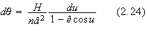
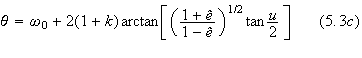
which
can be integrated to
![]()
where
![]() .
.
Looking at (2.18) and (2.20) one can see that
![]() has a minima (periastron passage) for
has a minima (periastron passage) for
![]() This, according to Damour and Deruelle, means that the periastron precesses by
the angle
This, according to Damour and Deruelle, means that the periastron precesses by
the angle
![]() at each turn ([5]).
at each turn ([5]).
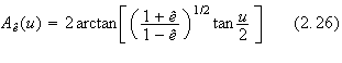
This section will not contain any derivations but only the result of
calculations made in [5]. By eliminating
![]() between (2.14) and (2.25) one can show that the relative orbit is given
by
between (2.14) and (2.25) one can show that the relative orbit is given
by
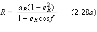
with
![]()
where
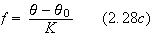
![]()
By using the solution for the relative motion,
![]() ,
,
![]() and
and
![]() in the post-Newtonian center off mass formulae we can obtain the expressions
for the relativistic motions of each body. Like in the preceding section this
one will not contain any derivations but just the resulting equations. The
result is
in the post-Newtonian center off mass formulae we can obtain the expressions
for the relativistic motions of each body. Like in the preceding section this
one will not contain any derivations but just the resulting equations. The
result is
![]()
where
The
orbit in space of one of the bodies can be described by
This
equation describes the
conchoid Note_3 of a precessing
ellipse.
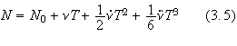
This section reviews the results of the timing formula presented by Damour and Deruelle in [6].
The timing formula is a formula linking the time of arrival
![]() of the Nth pulse emitted by a pulsar in a binary system to the integer N.
Introducing the time variables
of the Nth pulse emitted by a pulsar in a binary system to the integer N.
Introducing the time variables
![]() ,
,
![]() ,
,
![]() ,
,
![]() and
and
![]() will allow a derivation of a timing formula of the type
will allow a derivation of a timing formula of the type
![]()
![]()
![]()
![]()
![]()
![]()
Assuming that using
![]() one has computed the time of arrival
one has computed the time of arrival
![]() of the
N
of the
N![]() pulse at the barycenter of the solar system in absence of any solar
gravitational redshift and interstellar
dispersion Note_4 . We can
hereby define
pulse at the barycenter of the solar system in absence of any solar
gravitational redshift and interstellar
dispersion Note_4 . We can
hereby define
![]() to be the infinite-frequency barycenter arrival time.
to be the infinite-frequency barycenter arrival time.
Using a system of coordinates such that the barycenter of the binary system is
at rest at the origin we can compute the coordinate time of
arrival
![]() ,
a relation linking the proper time
,
a relation linking the proper time
![]() to the integer N. Here the barycenter of the solar system is moving with the
velocity
to the integer N. Here the barycenter of the solar system is moving with the
velocity
![]() and the relation (3.1b) is given by
and the relation (3.1b) is given by
![]()
In
this context, constants like the one above are unimportant and will be
neglected.
By using a coordinate position vector of the barycenter of
the solar system
![]() and a coordinate position vector of the pulsar
and a coordinate position vector of the pulsar
![]() (see figure 3), the coordinate time of arrival
(see figure 3), the coordinate time of arrival
![]() can be linked to the coordinate time of emission of
the pulse
can be linked to the coordinate time of emission of
the pulse
![]() by
by
![]()
where
![]() is the Shapiro time
delay Note_5 .
is the Shapiro time
delay Note_5 .
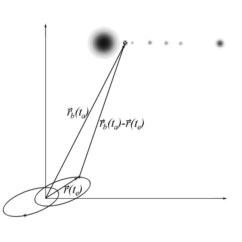
Figure 3: The coordinates of the barycenter
Now, to find the relation (3.1d), we first introduce a suitable proper time
![]() for the pulsar and a proper time
for the pulsar and a proper time
![]() for the emission of the Nth pulse. These two proper times are related
as
for the emission of the Nth pulse. These two proper times are related
as
![]()
where
![]() is the aberration time delay, a time delay associated to the angular shift of
the proper angle measuring the position of the emission spot which rotates
around the spin axis. This equation gives the time at which the Nth pulse
would have been emitted if the pulsar mechanism had been a radial pulsation
instead of a rotating beacon. From this fact, one finds that
is the aberration time delay, a time delay associated to the angular shift of
the proper angle measuring the position of the emission spot which rotates
around the spin axis. This equation gives the time at which the Nth pulse
would have been emitted if the pulsar mechanism had been a radial pulsation
instead of a rotating beacon. From this fact, one finds that
![]() is implicitly defined as a function of
is implicitly defined as a function of
![]() by the relation
by the relation
where
![]() is the proper rotation frequency of the pulsar (at
is the proper rotation frequency of the pulsar (at
![]() ).
The coordinate time of emission,
).
The coordinate time of emission,
![]() ,
is now linked to the proper time of emission
,
is now linked to the proper time of emission
![]() by
by
![]()
where
![]() is the Einstein time delay, a delay caused by the gravitational redshift due
to the companion and by the second order Doppler effect.
is the Einstein time delay, a delay caused by the gravitational redshift due
to the companion and by the second order Doppler effect.
By using equations (3.4), (3.6) and a Doppler factor
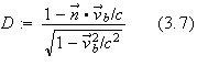
it
can be shown that
![]() is related to
is related to
![]() by
by
![]()
where
![]() is the Roemer time delay, i.e. the time of flight across the orbit counted
from the barycenter and projected on the line of sight. In this formula, the
order of magnitude of the four different time delays are
is the Roemer time delay, i.e. the time of flight across the orbit counted
from the barycenter and projected on the line of sight. In this formula, the
order of magnitude of the four different time delays are
![]()
We are using a center of mass frame such that the motion of the pulsar lies in
the plane
![]() .
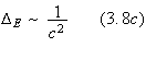
By choosing the plane of the sky to be
.
By choosing the plane of the sky to be
![]() the orientation of the center of mass frame with respect to this plane of the
sky are given by the two angles
the orientation of the center of mass frame with respect to this plane of the
sky are given by the two angles
![]() and
and
![]() where
where
![]() is the longitude of the ascending
node Note_6 and
is the longitude of the ascending
node Note_6 and
![]() is the inclination. The triad
is the inclination. The triad
![]() can be found from the reference triad
can be found from the reference triad
![]() by two successive rotations (illustrated in figure 4). First one rotates the
triad
by two successive rotations (illustrated in figure 4). First one rotates the
triad
![]() into a temporary triad
into a temporary triad
![]() by
by
![]()
![]()
![]()
Then,
by rotating this temporary triad as
![]()
![]()
![]()
one
ends up at the triad
![]() .
In this sense, the unit vector
.
In this sense, the unit vector
![]() is directed towards the ascending node
is directed towards the ascending node
![]() and
and
![]() is pointing from the Earth to the orbit of the
pulsar.
is pointing from the Earth to the orbit of the
pulsar.
Figure 4: Angular elements of the pulsar orbit
By using planar polar coordinates and looking back at equations (2.13), (2.14)
and (2.25) one can find a parametric representation of the motion of the
pulsar given by
![]()
![]()
![]()
where
![]() are constants. Using equation (3.6) with (3.11) leads to a relation between
the eccentric anomaly parameter
are constants. Using equation (3.6) with (3.11) leads to a relation between
the eccentric anomaly parameter
![]() and the proper time
and the proper time
![]() :
:
![]()
where
![]() is a modified expression given by
is a modified expression given by
![]()
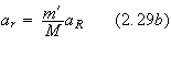
with
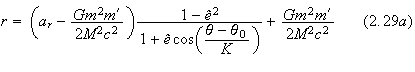
Here
![]() is given by equation (2.29b).
is given by equation (2.29b).
The parametric representation of the motion of the pulsar expressed in proper
time
![]() is now given by the equations (3.14), (3.12) and (3.13), so what is left now
is to find an explicit timing formula. This turns out to be quite complicated
and will thus not be presented in this project. The interested reader is
recommended to have a look at [6].
is now given by the equations (3.14), (3.12) and (3.13), so what is left now
is to find an explicit timing formula. This turns out to be quite complicated
and will thus not be presented in this project. The interested reader is
recommended to have a look at [6].
The theory of General Relativity, postulated by Einstein, describes the gravitational force as a consequence of the curvature of space-time. This curvature is caused by massive objects; the more massive an object is, the greater curvature it causes and the more intense the gravity is. A massive object, like a member of a binary system, rotating around its companion will cause ripples in space-time, just like the ripples in a lake. These ripples are referred to as gravitational waves. As these waves evolves through the universe, space-time will distort in a peculiar way. The distance between objects will increase and decrease rhythmically as the wave passes by. This effect is not very big though, not even detected yet.
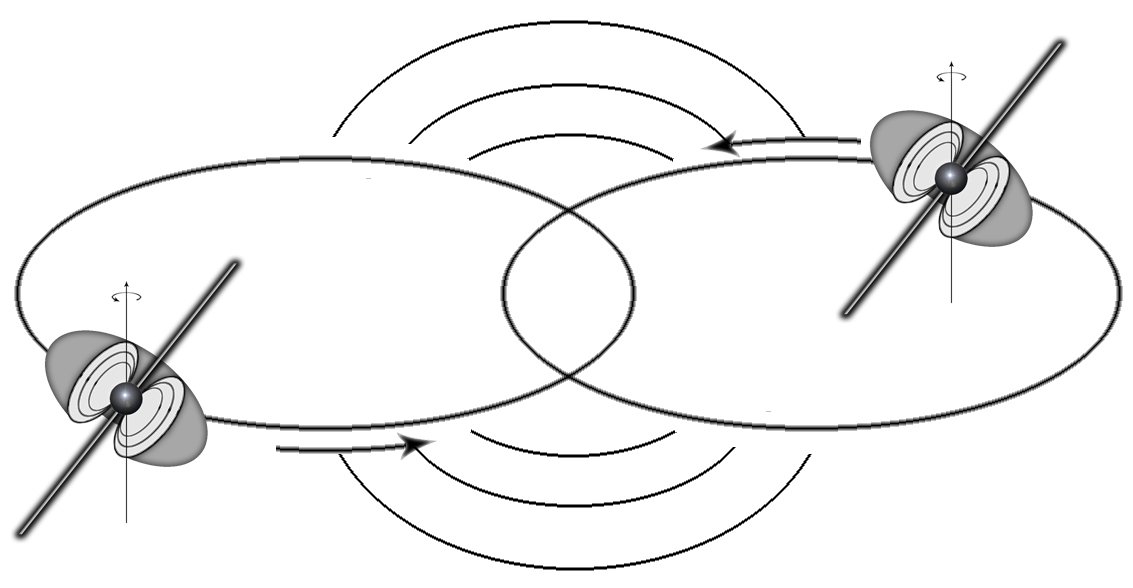
Figure 5: Gravitational Waves.
One important source of radiation is the Hulse-Taylor binary PSR1913+16, a binary system of two stars, one of which is a pulsar and the other probably an ordinary neutron star. Here one pulsar year is only about eight hours and, by observing the shift in the pulses, the stars are found to be equally heavy, each weighing about 1,4 times as much as the Sun. As the energy is carried away from the binary by the gravitational wave, the orbits will converge and with time the members will collide. This kind of orbit is called an inspiral and can be observed by the pulsar timing of the system. These observations are the first indirect evidence for gravitational waves but a more interesting observation would be a direct evidence. This would provide us with a rigorous test of the theory of General Relativity and also information about things we cannot see with electromagnetic radiation, like black holes. Nevertheless, the weak nature of gravitational radiation makes it very difficult to design a sensitive detector filtering out the noisy background. Various detectors are though in use and we expect a result to appear in a near future. There is a lot more to learn about gravitational waves and for the reader interested in an introduction to the topic I recommend to have a look at [4].
In section 2, we reviewed the main parts of the method for solving the
post-Newtonian motion in the post-Newtonian mass frame. We found the
parametric solution to be
![]()
![]()
![]()
![]()
where
and
![]() are given in terms of the total energy and the total angular momentum.
are given in terms of the total energy and the total angular momentum.
In section 3, we reviewed the motion of the pulsar expressed in proper time
![]() which are given in a parametric form by
which are given in a parametric form by
![]()
![]()
where
![]()
and
![]() are constants.
are constants.
[1] Freedman and Kaufmann, Universe,
7![]() edition, New York, W. H. Freeman and Company, 2005
edition, New York, W. H. Freeman and Company, 2005
[2]
Goldstein, Poole and Safko, Classical Mechanics,
3![]() edition, San Fransisco, Pearson Education, 2002
edition, San Fransisco, Pearson Education, 2002
[3] Infeld
and Plebanski, Motion and Relativity, Pergamon, Oxford,
1960
[4] Chakrabarty, Gravitational Waves:
An Introduction, Retrieved December, 2006, from
http://arxiv.org/PS_cache/physics/pdf/9908/9908041.pdf
[5]
Damour and Deruelle, General relativistic celestial mechanics
of binary systems. I. The post-Newtonian motion, Retrieved December,
2006,
from
http://luth2.obspm.fr/IHP06/lectures/damour/DamourDeruelleAIHP85.pdf
[6]
Damour and Deruelle, General relativistic celestial mechanics
of binary systems. II. The post-Newtonian timing formula, Retrieved
December, 2006, from
http://luth2.obspm.fr/IHP06/lectures/damour/DamourDeruelleAIHP86.pdf
[7]
Lorimer, Binary and Millisecond Pulsars, Retrieved
December, 2006, from
http://relativity.livingreviews.org/Articles/lrr-2005-7/
[8]
Conchoid (mathematics), Retrieved December, 2006,
from
http://en.wikipedia.org/wiki/Conchoid_%28mathematics%29
[9]
Eccentric anomaly, Retrieved December, 2006,
from
http://en.wikipedia.org/wiki/Eccentric_anomaly
[10]
Gravity Probe B, Retrieved December, 2006,
from
http://einstein.stanford.edu/
[11]
Gravitational wave, Retrieved December, 2006,
from
http://en.wikipedia.org/wiki/Gravitational_waves
[12]
The Nobel Prize in Physics 1993, Retrieved December,
2006,
from
http://nobelprize.org/nobel_prizes/physics/laureates/1993/illpres/discovery.html
All images have been produced by the author.